Our economy is populated by a large number of households , the utility function of the representative household is defined by:

where is the risk aversion and is the frischian elasticity of labor. is increasing in consumption and decreasing with hours worked .

The welfare index is determined by the sum of the current and expected utilities:

Additionally, the production function follows a Cobb-Douglas technology:

where is an IID exogenous disturbance associated with a productivity shock.
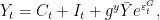
The resources constraint is given by the demand from households and authorities:

where is a IDD normal shock, is the steady state level of the GDP and is the spending to GDP ratio.

Capital law of motion reads as in Solow’s model and is determined by:

The Cobb-Douglas production function now combines labor, physical capital and technology to produce goods:

where is an IID exogenous disturbance associated with a productivity shock.
The resources constraint now includes investment:

where is a IDD normal shock, is the steady state level of the GDP and is the share of public spending to the GDP.

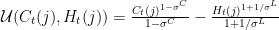
In this setting, we consider that each household has external consumption habits. This feature captures the autocorrelation of consumption observed in the data. Thus the utility function subject to external habits reads as follows:

To introduce asset price fluctuations, households supplying investment goods face an investment adjustement costs given by:

The law of motion of capital with investment adjustment costs is defined by:

These costs drive a wedge between the price of assets and goods and offer a tradeoff beetwen capital goods and riskless bonds.

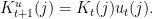
Standard RBC model suppose that capital is homogenous and its utilization is constant. CEE (2005) introduce variable capital utilization in order to match the data. The amount of capital utilized in the production is:

This equation shows that capital requires one period to be installed (i.e; “time to build”).
The Cobb-Douglas production function now combines technology, labor and utilized capital:

The variable utilization of capital incurs a variable cost, denoted . Its functional forms is defined by:
$altex a(u_t) = \bar{Z}(u_t-1) + \frac{\bar{Z}}{2}\frac{\psi}{1-\psi}(u_t-1)^2.$
Given this cost, the resources constraint also includes capital utilization costs:

In equilibrium, the optimal capital utilization is defined by:

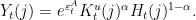
The standard New Keynesian model assumes that monopolistic competitive firms are price makers on the good market, but they cannot adjust prices as prices are sticky. There are two ways of introducing nominal rigidities: the Rotemberg way, see Rotemberg (1982) and the Calvo price setting, see Calvo (1983). I present here the Calvo price setting. There is a continuum of monopolitic firms that chooses their price $P^* _t(i)$. Among these firms, a fraction is not allowed to set price, then the price remains the same such that . For the share of firms allowed to reset their price, each firm maximizes the expected sum of profits:

under the demand constraint from final goods packers.
The FOC from the previous problem, combined with the aggregate price equation and taken in logs gives rise to the New Keynesian Phillips Curve (NKPC):

Finally, to close the model, we suppose that monetary authority controls the nominal interest rates and is concerned by both price and GDP growths. The monetary policy rule à la Taylor in logs reads:

Galì and Gertler (1999) observe backward looking dynamics in firms’ price setting. They include in New Keynesian setup an indexation mechanism when firms are setting their price. In particular in our model, for the fraction of firms not allowed to reset price, their selling price remains the same such that and indexed on past inflation in a proportion . Concerning the share of firms allowed to reset their price, each firm maximizes the expected sum of profits:

under the demand constraint from final goods packers.
The FOC from the previous problem, combined with the aggregate price equation and taken in logs give rise to the New Keynesian Phillips Curve (NKPC):
$late
\widehat{\pi}_t = \gamma^p\widehat{\pi}_{t-1} + \beta E_t\widehat{\pi}_{t+1} + \frac{(1-\theta^p)(1-\beta\theta^p)}{\theta^p}(\widehat{mc}_t-\widehat{p}_t).

This paper questions the role of cross-border lending in the definition of national macroprudential policies in the European Monetary Union. We build and estimate a two-country DSGE model with corporate and interbank cross-border loans, Core-Periphery diverging financial cycles and a national implementation of coordinated macroprudential measures based on Countercyclical Capital Buffers. I provide here the estimated model (at the mode), not the optimization exercise.

In this paper published in Revue d’Economie Politique in 2017, we estimate DSGE model of the European Monetary Union that accounts for financial differences between core and peripheral countries. We find that country-adjusted macroprudential measures lead to significant welfare gains with respect to a uniform macroprudential policy rule that reacts to union-wide financial developments. However, peripheral countries are the winners from the implementation of macroprudential measures while core countries incur welfare losses, thus questioning the interest of adopting coordinated macroprudential measures with peripheral countries.

In this paper published in Research in Economics in 2015, we evaluate the role of financial frictions on the decision to create new goods/startups using an estimated DSGE model. We extend the initial framework of Bilbiie, Ghironi and Melitz (2012) and augment it with real, nominal and financial frictions to get a data friendly model. The model is estimated using Bayesian techniques for the US economy. I share the model which is calibrated on the posterior estimated mean value of deep parameters and shocks, I also share the data involved in the estimation exercise.

This code was published in the Economics and Business Review hosted by the University of Poznan. This paper aims at introducing New Keynesian Macroeconomics for graduate students. This paper is currently taught in the Master Program of the University Paris-Dauphine, University of Rennes and the University of Poznan.

Bibliography

Melitz, M., Bilbiie, F. O., & Ghironi, F. (2012). Endogenous Entry, Product Variety, and Business Cycles. Journal of Political Economy, 120(2).
Calvo, G. A. (1983). Staggered prices in a utility-maximizing framework. Journal of monetary Economics, 12(3), 383-398.
Christiano, L. J., Eichenbaum, M., & Evans, C. L. (2005). Nominal rigidities and the dynamic effects of a shock to monetary policy. Journal of political Economy, 113(1), 1-45.
Poutineau, J. C., & Vermandel, G. (2015). Cross-border banking flows spillovers in the Eurozone: Evidence from an estimated DSGE model. Journal of Economic Dynamics and Control, 51, 378-403.
Poutineau, J. C., & Vermandel, G. (2015). Financial frictions and the extensive margin of activity. Research in Economics, 69(4), 525-554.
Poutineau, J. C., & Vermandel, G. (2017). A Welfare Analysis of Macroprudential Policy Rules in the Euro Area. Revue d Economie Politique.
Poutineau, J. C., & Vermandel, G. (2017). Global banking and the conduct of macroprudential policy in a monetary union. Journal of Macroeconomics, 54, 306-331.
Rotemberg, J. J. (1982). A monetary equilibrium model with transactions costs.
Smets, F., & Wouters, R. (2003). An estimated dynamic stochastic general equilibrium model of the euro area. Journal of the European economic association, 1(5), 1123-1175.
Smets, F., & Wouters, R. (2007). Shocks and frictions in US business cycles: A Bayesian DSGE approach. National bank of belgium working paper, (109).